Students access the ice core data archived at Lamont-Doherty Geological Observatory. They select a core (Greenland, Antarctica, Quelcaya), pose a working hypothesis regarding the data, import the data in an Excel-readable format, and examine the data to determine correlations between variables and cause/effect as recorded in leads and lags. They generate a written and graphical analysis of the data and, in the next lab period, discuss the similarities and differences among their group outputs in terms of demonstrated correlations, assumptions required, effects of latitude, and any other item that arises.

(Note: this resource was added to OER Commons as part of a batch upload of over 2,200 records. If you notice an issue with the quality of the metadata, please let us know by using the 'report' button and we will flag it for consideration.)

The transgressive coastal sequence, as a fundamental concept in stratigraphy, will be explored by the students in a hands-on activity based on a set of high-resolution seismic profiles collected in the shoreface off Assateague Island, Maryland and Virginia. Small groups of 2-3 students will identify primary surfaces, such as the ravinement surface and sequence boundaries, and major sedimentary facies, such as offshore shoals, flood-tidal deltas, and tidal inlets, in a set of shore-parallel and shore-perpendicular lines. The exercise begins with factors controlling relative sea level and leads into accommodation space and preservation potential.

(Note: this resource was added to OER Commons as part of a batch upload of over 2,200 records. If you notice an issue with the quality of the metadata, please let us know by using the 'report' button and we will flag it for consideration.)

In this exercise, students use whole-rock major- and trace-element compositions of igneous rocks from a variety of tectonic settings and locations to explore the importance of plate setting in determining magma compositions. Students are split into groups and assigned different tectonic settings to examine and compare with other groups. Datasets are obtained from the GEOROC database, imported into Excel spreadsheets, and graphed to learn how igneous rock compositions are a function of plate tectonic setting.

(Note: this resource was added to OER Commons as part of a batch upload of over 2,200 records. If you notice an issue with the quality of the metadata, please let us know by using the 'report' button and we will flag it for consideration.)

In this exercise, students are split into groups to gather whole-rock geochemical data (major-, trace-, and rare-earth elements) from the GEOROC database for igneous rocks sampled from four different plate tectonic settings: mid-ocean ridges, subduction zones, oceanic islands, and oceanic plateaus. Each group is assigned a different plate tectonic setting and collects three datasets from different locations for their tectonic setting. Geochemical data is graphed as major-element variation and REE diagrams to quantify igneous diversity both within the same tectonic setting and between different tectonic settings. The main goal of this exercise is to demonstrate that igneous rock compositions are a strong function of plate tectonic setting.

(Note: this resource was added to OER Commons as part of a batch upload of over 2,200 records. If you notice an issue with the quality of the metadata, please let us know by using the 'report' button and we will flag it for consideration.)

Quick review worksheet that has students draw a sequence of illustrations of what would occur to a syntectonic quart vein, a pebble conglomerate, a rigid object, and a garnet porphyroblast for pure vs. simple shear. I've used this both as a quiz & as an in-class review.

(Note: this resource was added to OER Commons as part of a batch upload of over 2,200 records. If you notice an issue with the quality of the metadata, please let us know by using the 'report' button and we will flag it for consideration.)

Short in-class review question about using given strike and dip information to classify a fold. Stereonets used.

(Note: this resource was added to OER Commons as part of a batch upload of over 2,200 records. If you notice an issue with the quality of the metadata, please let us know by using the 'report' button and we will flag it for consideration.)

A toddler wading pool or similar tank is filled with common sand (available from home improvement stores in bags) to a depth of 15-20 cm. The sand is saturated with a slow inflow and outflow to a floor drain. A 2-inch PVC slotted screen section is buried in the sand near the center of the tank with a capped end at the bottom. Small (1 cm diameter or similar) slotted or perforated PVC or copper tubing are placed as piezometers in the sand at short distances (e.g., 10-20 cm) from the pumping "well." A fountain pump capable of discharging up to 100-150 ml/min is placed within the "well" with adequate discharge tubing to conduct the water to a drain. A stopcock is placed in the tubing to control flow. Alternatively, if the tank of sand is on a very sturdy table, a simple siphon with tubing can be used as a pump. Drawdown is determined by the difference between a pre-pumping level measurement from the top of the "piezometers" and subsequent measurements made in the same "piezometer" at times after pumping starts. Water levels may be measured using chalked wooden rods. Alternatively, a small cork with a slender wooded food skewer marked in millimeter increments can be placed in each piezometers and the students can watch the change in level of the markings relative to the top of the "piezometer." Flow is repeatedly measured using a graduated cylinder. At the start of the test, students or teams of students are assigned to either take water level measurements at a specific piezometer or to measure and control the flow rate. The data are collected on a logarithmically increasing time interval for about an hour. The flow and drawdown data are analyzed by various means (Theis curve, Jacob straight-line method, Bolton curves, etc.) either manually or using AQTESOLV or similar software. Though the drawdowns are small, the data have provided quite reasonable estimates of hydraulic conductivity for the sand.

(Note: this resource was added to OER Commons as part of a batch upload of over 2,200 records. If you notice an issue with the quality of the metadata, please let us know by using the 'report' button and we will flag it for consideration.)

This module includes 10 topics related to finding, evaluating, and presenting scientific information related to climate change or other interdisciplinary topics.

The ultimate goal is for students to prepare a paper and present it to their colleagues as though they were giving it at typical professional meeting such as American Geophysical Union, Geological Society of America, or American Quaternary Association. However, the technical level of the talk should be at a level that the class will understand and enjoy.

The topic should demonstrate scientific method rather than being merely descriptive or primarily applied science/technology. Students should use current literature. The presentation will be more interesting if the subject is somewhat controversial. The final product should demonstrate that the student understands and has gained the skills presented in all 10 topics.

(Note: this resource was added to OER Commons as part of a batch upload of over 2,200 records. If you notice an issue with the quality of the metadata, please let us know by using the 'report' button and we will flag it for consideration.)

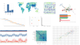
Information visualization is concerned with the visual and interactive representation of abstract and possibly complex datasets. As we encounter growing datasets in various sectors there is an increasing need to develop effective methods for making sense of data. Information visualization relies on computational means and our perceptual system to help reveal otherwise invisible patterns and gain new insights. Across various fields, there is great hope in the power of visualization to turn complex data into informative, engaging, and maybe even attractive forms. However, it typically takes several steps of data preparation and processing before a given dataset can be meaningfully visualized. While visualizations can indeed provide novel and useful perspectives on data, they can also obscure or misrepresent certain aspects of a phenomenon. Thus it is essential to develop a critical literacy towards the rhetoric of information visualization. One of the best ways to develop this literacy is to learn how to create visualizations! The tutorials offer a practical approach to working with data and to create interactive visualizations.

The tutorials require basic familiarity with statistics and programming. They come as Jupyter notebooks containing both human-readable explanations as well as computable code. The code blocks in the tutorials are written in Python, which you should either have already some experience with or a keen curiosity for. The tutorials make frequent use of the data analysis library Pandas, the visualization library Altair, and a range of other packages. You can view the tutorials as webpages, open and run them on Google Colab, or download the Jupyter notebook files to edit and run them locally.

To illustrate the basics of digital mapping on a PocketPC, I have included one of the projects used in our field course. It covers an area southeast of Buena Vista, Colorado that consists of Precambrian plutonic and metamorphic rocks, Tertiary volcanic rocks, and Quaternary sediments. The project comes in the second week of the course and is the first digital mapping experience for the students. Prior to this, they have been learning to map using traditional methods.
The Sugarloaf project consists of base maps and data layers. The inclusion of both aerial photo (USGS DOQQ) and topographic base maps (USGS DRG), allows students to choose which ever map works best for them. The data layers include everything that a field geologist would normally record in his/her field notebook and map: general notes, contacts, and structural data (including oriented symbols on the map). The specific layers in this project are: bedding, contacts, faults, foliations, formations, geology, joints, lineations, and stations. In some layers (e.g., bedding, foliation, lineation, and joint), taping a point on the map opens a dialog box into which you enter data such as strike/dip or plunge/trend. In other layers (e.g., stations), taping a point opens a form for notes. In the contact layer, you draw lines. Editing can be done in the field on your PocketPC or back in camp by downloading the project to a computer. If a project is edited on a computer, the edited version must then be uploaded to the PocketPC for use the next day in the field. Final production of the map is done using ArcView or ArcMap.

(Note: this resource was added to OER Commons as part of a batch upload of over 2,200 records. If you notice an issue with the quality of the metadata, please let us know by using the 'report' button and we will flag it for consideration.)

This is a short project that can be used in-class or as homework. It involves just a few questions and it is intended to help students understand the idea of Gibbs free energy. It cannot completely stand alone. I use it after I have talked about Gibbs free energy for 20 minutes. It helps clarify my lecture.

(Note: this resource was added to OER Commons as part of a batch upload of over 2,200 records. If you notice an issue with the quality of the metadata, please let us know by using the 'report' button and we will flag it for consideration.)

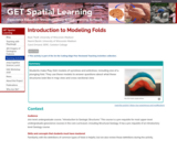
Play-Doh model, upright anticline

Provenance: Carol Ormand Ph.D., Carleton College
Reuse: This item is offered under a Creative Commons Attribution-NonCommercial-ShareAlike license http://creativecommons.org/licenses/by-nc-sa/3.0/ You may reuse this item for non-commercial purposes as long as you provide attribution and offer any derivative works under a similar license.
Students make Play-Doh models of synclines and anticlines, including one of a plunging fold. They use these models to answer questions about what these structures look like in map view and cross-sectional view.

(Note: this resource was added to OER Commons as part of a batch upload of over 2,200 records. If you notice an issue with the quality of the metadata, please let us know by using the 'report' button and we will flag it for consideration.)

This book is an introduction to the language of systems biology, which is spoken among many disciplines, from biology to engineering. Authors Thomas Sauter and Marco Albrecht draw on a multidisciplinary background and evidence-based learning to facilitate the understanding of biochemical networks, metabolic modeling and system dynamics.

Their pedagogic approach briefly highlights core ideas of concepts in a broader interdisciplinary framework to guide a more effective deep dive thereafter. The learning journey starts with the purity of mathematical concepts, reveals its power to connect biological entities in structure and time, and finally introduces physics concepts to tightly align abstraction with reality.

This workbook is all about self-paced learning, supports the flipped-classroom concept, and kick-starts with scientific evidence on studying. Each chapter comes with links to external YouTube videos, learning checklists, and Integrated real-world examples to gain confidence in thinking across scientific perspectives. The result is an integrated approach that opens a line of communication between theory and application, enabling readers to actively learn as they read.

This overview of capturing and analyzing the behavior of biological systems will interest adherers of systems biology and network analysis, as well as related fields such as bioinformatics, biology, cybernetics, and data science.

This exercise gives students personal experience with data sets that have spatial reference "issues" so that they learn first hand both why it matters to be meticulous about projections and coordinate systems and how to work with coordinate systems, projections, and datum transformations in ArcMap. You might also be interested in our Full GIS course with links to all assignments.

Students map the classroom twice using paper and pencil, the first time on different pieces of paper and with essentially no instructions and the second time on a base map with coordinates for one corner of the room with instructions about what to map and make a table of information about what they are mapping. *Special thanks to Dennis Johnson, Juniata College, for the basic idea for this activity!* You might also be interested in our Full GIS course with links to all assignments.

This exercise uses a suite of well logs (aka electric logs) to interpret lithology within a stratigraphic section and to determine fluid content within borehole rocks.

This series of three activities in tutorial format serves not only as an introduction to ArcGIS for our intro geology, hydrogeology, and structural geology courses but also as a mandatory refresher that students must complete before the first lab of our upper level course GIS for Geoscientists. The tutorial/refresher emphasizes techniques used by geoscientists. You might also be interested in our Full GIS course with links to all assignments.

After exposure to the basic concepts of biostratigraphy and magnetostratigraphy, participants apply these concepts to produce a biomagnetostratigraphic age model using microfossil and paleomagnetic data from a Paleogene core recovered from Walvis Ridge in the South Atlantic (Ocean Drilling Program Site 1262). The investigation has three parts: First, observed first and last occurrences of various planktonic foraminifera species at different core depths are given absolute ages through reference to the Berggren et al. (1985) time-scale. Second, these planktonic foraminiferal data are used to identify magnetic reversals within the same core and thereby assign absolute ages to these events. Third, the resulting biomagnetostratigraphic age model is used to estimate the time between two well-documented "hyperthermals" within the core, the Paleocene-Eocene Thermal Maximum (PETM) and the Eocene Layer of Mysterious Origin (ELMO). The investigation illustrates how biostratigraphy and magnetostratigraphy complement one another and together provide an operational time-domain for all subsequent studies, be they paleoceanographic, evolutionary, etc. Note that this investigation operates on an established timescale (i.e., Berggren et al, 1985) and does not explictly demonstrate how such timescales are developed. Thus, instructors are encouraged to have students construct a simple composite relative time scale from basic outcrop data prior to this investigation.

(Note: this resource was added to OER Commons as part of a batch upload of over 2,200 records. If you notice an issue with the quality of the metadata, please let us know by using the 'report' button and we will flag it for consideration.)

Students will write a matlab code to calculate crustal thickness of 5 locations. Calculations will use topography (determined by running a matlab script that creates a clickable map) and nominal density values, and the assumption that the crust is in airy isostasy. Students will then run another script (with clickable map) to determine the actual crustal thickness of the locations. If the calculated and actual thicknesses are significantly different, students will discuss possible geodynamic reasons for the non-airy crustal thicknesses.